The Statistics of Changing Uncertainty

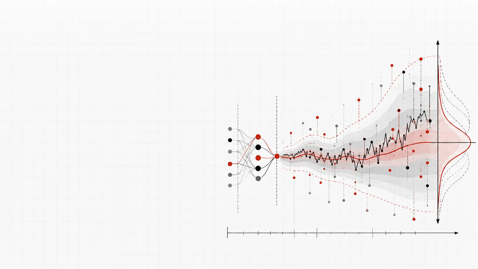
Suppose your model says tomorrow will probably look like today. A perfectly respectable forecast. Then an unexpected announcement arrives, prices lurch, and your beautifully fitted curve becomes a historical document.

The tempting response is to blame randomness. The more useful response is to ask what the model assumed about it. Did we allow the level of uncertainty to change, or did we quietly give every day the same variance and hope the world would cooperate?

That question connects statistical physics, the Gamma distribution, and neural networks. Quantum ideas enter too, although they need a more specific job description than “everything is unpredictable, therefore quantum.”

The average looks fine

Imagine two weeks of market returns. One is quiet. The other features large gains and losses that nearly cancel out. Both can have an average close to zero. Only one makes you check your portfolio during dinner.

Financial returns often exhibit volatility clustering: large movements tend to occur near other large movements. Their distributions also tend to have heavy tails, giving extreme movements more probability than a Normal distribution with comparable variance would suggest. Rama Cont (2001) documents these recurring properties across financial datasets.

One possible explanation involves mixing different risk environments. A narrow distribution might describe a calm period reasonably well. A turbulent period needs a wider one. Combine those periods, and the resulting distribution can contain more extreme observations than a single Normal model would suggest.

Even variance does not tell the whole story. Two distributions can share a mean and variance while disagreeing substantially about how often a really unpleasant day should occur.

Physics has a framework for this

Beck and Cohen (2003) introduced superstatistics to describe systems whose local behaviour depends on a fluctuating parameter, such as inverse temperature. Conditions remain approximately stable locally, while the environmental parameter changes more slowly. Averaging across those conditions produces the overall distribution.

Consider your commute. Travel time varies even under ordinary traffic conditions. Rush hour changes the conditions themselves. Pool every journey into one dataset, and a single distribution must account for both sources of variation. The navigation app's confidence may be admirable; your arrival time remains less committed.

The statistical distinction is between a conditional distribution, describing outcomes given the current state, and a marginal distribution, combining possible states. Superstatistics also requires a separation of time scales: local behaviour adjusts faster than the environmental parameter changes. Beck, Cohen, and Swinney (2005) explain how to investigate that assumption in observed series.

Gamma earns its place in the equation

Let $X$ represent a return after removing its conditional location. Assume it is Normally distributed given a positive parameter $\tau$, called precision. Precision is the reciprocal of variance, so smaller precision means greater uncertainty. Now let precision itself follow a Gamma distribution:

Here $\alpha$ is the shape and $\beta$ the rate, both positive. Gamma is a candidate because precision must be positive. Returns, which can be negative, require a different role in the model. Giving everything a Gamma distribution would certainly simplify the paperwork.

To obtain the overall return distribution, average over possible precision values. This is marginalization, the integral doing the bookkeeping for an unobserved quantity:

The result is Student's $t$. Changing uncertainty has produced heavy tails from conditionally Normal behaviour. At fixed mean precision, smaller $\alpha$ means greater relative variation in precision and heavier tails. The scale above is not the standard deviation: when $\alpha>1$, the variance is $\beta/(\alpha-1)$.

For perspective, compare a Normal variable with a Student's $t$ variable having five degrees of freedom, rescaled to the same mean and variance. Across 1,000 observations, their theoretical expected counts beyond three standard deviations are roughly three and twelve, respectively. Same variance; very different reasons to worry.

That calculation illustrates the assumptions, rather than validating them. Xu and Beck (2016) found that chi-square superstatistics, involving a special case of Gamma, worked well for daily returns in their data. At minute intervals, a Lognormal form worked better. An elegant derivation still has to survive a meeting with the dataset.

A neural network gets a more useful assignment

A Gamma distribution alone cannot tell us whether today's turbulence will persist tomorrow. It describes possible precision values, not their temporal dependence. Forecasting needs an additional model of how conditions evolve.

A neural network could learn from past observations to predict the parameters of tomorrow's distribution. DeepAR demonstrates the broader approach of probabilistic forecasting with recurrent neural networks (Salinas et al., 2020). Using a network with the particular Gamma mixture above is a modelling proposal, rather than a finding established by DeepAR.

The output could answer a practical question: what is the probability that a business's dollar payment exceeds its budget next month? That is more useful for planning than an expected exchange rate presented to four decimal places, as though the fourth decimal had signed a contract.

There is a statistical catch. The Normal-Gamma mixture produces Student's $t$, so predicting its Gamma parameters is equivalent to predicting the corresponding $t$ parameters directly. A change of notation creates no extra information. Any forecasting improvement must come from the learned relationships or useful modelling constraints.

Quantum needs a specific role

So far, the connection belongs to probability and statistical physics. A separate connection concerns training the network.

Training searches for weights that reduce a loss function. Picture a landscape where height represents error. Quantum annealing uses quantum effects, including tunneling, to explore optimization problems. Ohzeki and colleagues (2018) investigated retaining finite quantum fluctuations at the final stage of a network optimization method. They reported improved generalization in their experiments, while computational constraints limited large-scale testing.

This gives quantum ideas a documented role in learning. It provides no evidence that market volatility is driven by quantum fluctuations, or that such training predicts geopolitical crises. The word “quantum” has already been asked to do enough unpaid work.

The forecast still has to earn our trust

A probabilistic model should be tested on later observations unavailable during training. Its probabilities also need calibration: across many comparable cases assigned a 10% probability, the event should occur roughly one time in ten. Proper scoring rules, including the logarithmic score and continuous ranked probability score, help evaluate complete predictive distributions (Gneiting & Raftery, 2007).

Global events demand their own definitions, time horizons, and relevant data. Explaining a heavy-tailed return distribution does not establish when a conflict or supply disruption will happen.

What these connections offer is a way to represent changing uncertainty explicitly and learn whether its changes contain useful signals. A wider prediction interval may look less impressive than a confident number. For someone making a real decision, knowing how much confidence the number deserves can be the more valuable forecast.

References

Cont, R. (2001). Empirical properties of asset returns: Stylized facts and statistical issues. Quantitative Finance, 1(2), 223–236. DOI.

Beck, C., & Cohen, E. G. D. (2003). Superstatistics. Physica A: Statistical Mechanics and its Applications, 322, 267–275. DOI00019-0).

Beck, C., Cohen, E. G. D., & Swinney, H. L. (2005). From time series to superstatistics. Physical Review E, 72(5), 056133. DOI.

Xu, D., & Beck, C. (2016). Transition from lognormal to chi-square superstatistics for financial time series. Physica A: Statistical Mechanics and its Applications, 453, 173–183. DOI.

Salinas, D., Flunkert, V., Gasthaus, J., & Januschowski, T. (2020). DeepAR: Probabilistic forecasting with autoregressive recurrent networks. International Journal of Forecasting, 36(3), 1181–1191. DOI.

Ohzeki, M., Okada, S., Terabe, M., & Taguchi, S. (2018). Optimization of neural networks via finite-value quantum fluctuations. Scientific Reports, 8, 9950. DOI.

Gneiting, T., & Raftery, A. E. (2007). Strictly proper scoring rules, prediction, and estimation. Journal of the American Statistical Association, 102(477), 359–378. DOI.