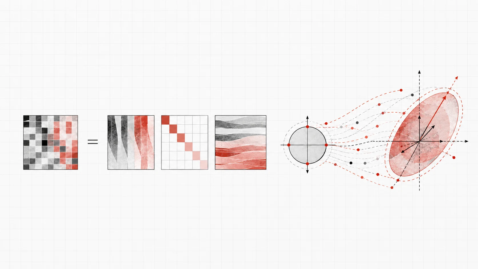
The Summit
Talking about SVD in linear algebra can feel like jumping straight to the top of a mountain. Why begin at the highest point of the theory before we know the path that leads there?
Do not worry. We are not going to memorize the summit or disappear into a maze of proofs. We will stand there for a moment, then take it apart until we can see what the mountain is made of.
From to
Since the story is about decomposition, begin in the opposite direction: composition.
Put three in front of us, , , and . Their dimensions fit, so we can connect them:
That is composition in its simplest form: we know the pieces, we combine them, and a new object appears. If a enters the chain, the action begins on the right:
so
Take a small numerical example:
Together they become
Figure 1: Matrix Composition as Sequential Transformations. The product ABC acts on x from right to left: C transforms the input first, followed by B and A.
Composition in Python
import numpy as np A = np.array([[1., 2.], [0., 1.]]) B = np.array([[2., 0.], [0., 0.5]]) C = np.array([[0., -1.], [1., 0.]]) W = A @ B @ Cprint(W)This is the forward direction: known pieces produce a final matrix.
Here you can touch composition instead of merely reading its definition. Change , press the matrices, and watch the vector move through , then , then .
Now reverse the question.
Instead of giving you the pieces, I place one matrix in front of you. We can inspect its rows and columns, calculate its , and measure everything visible from the outside. Then I say: open it. Show me the structure hiding inside.
Without a method, we could guess until the stars burn out. That is precisely why linear algebra developed decompositions: we do not want arbitrary factors; we want pieces with structure and jobs we can name.
The pieces may be , as in LU; directions plus triangular coefficients, as in QR; or one triangular factor mirrored by its , as in Cholesky. Sometimes we change the viewpoint itself, as in spectral decomposition and Schur. Sometimes we separate rotation from stretching, as in the polar decomposition. Then we reach SVD, which takes the stage from here.
The Decomposition Atlas
There are many names, but one instinct connects them: do not fight the matrix in the form in which it arrived. Find a representation in which each piece has a clear job.
In the interactive atlas below, choose LU, QR, Cholesky, Spectral, or SVD. Open the factors, then rebuild the original matrix. Do not memorize five formulas; watch the same move repeat.
LU turns Gaussian elimination into reusable matrix factors.
| 4 | 3 |
| 6 | 3 |
| 1 | 0 |
| 1.5 | 1 |
| 4 | 3 |
| 0 | -1.5 |
Lower triangular: it stores the elimination multipliers.
Figure 2: Matrix Factorization Methods. Five factorizations represent the same matrix through different structures, with each set of factors providing a route to reconstruct A.
A Small Decomposition Atlas in Python
import numpy as np A = np.array([[4., 2.], [2., 3.]]) # QRQ, R = np.linalg.qr(A)print(np.allclose(A, Q @ R)) # SVDU, s, Vt = np.linalg.svd(A)Sigma = np.diag(s)print(np.allclose(A, U @ Sigma @ Vt)) # Spectral decomposition for symmetric Alam, E = np.linalg.eigh(A)print(np.allclose(A, E @ np.diag(lam) @ E.T)) # Cholesky for positive-definite AL = np.linalg.cholesky(A)print(np.allclose(A, L @ L.T))With SciPy:
import numpy as npfrom scipy.linalg import lu, schur, polar A = np.array([[4., 2.], [2., 3.]]) P, L, U_lu = lu(A)T, Z = schur(A)Qp, H = polar(A) print(np.allclose(A, P @ L @ U_lu))print(np.allclose(A, Z @ T @ Z.T))print(np.allclose(A, Qp @ H))From here, SVD no longer feels like a jump into a different chapter. It is simply the decomposition we are about to examine more closely than the others.
The Essence, Nothing More
For any real matrix
we can write
In the full picture, is an matrix, is an orthogonal matrix, and is an matrix.
On the diagonal of sit the :
The columns of are the right singular vectors; the columns of are the left singular vectors. For complex matrices, is replaced by the .
Input vector
Choose a vector to transform.
Figure 3: Vector Transformation under the SVD. The factorization separates a vector transformation into an orthogonal change of coordinates by Vᵀ, scaling by Σ, and reorientation by U.
That is the formula. The meaning appears when each factor gets a job.
Compute and Check an SVD
import numpy as np A = np.array([[3., 1.], [1., 2.]]) U, s, Vt = np.linalg.svd(A)Sigma = np.diag(s) print("U =\n", U)print("singular values =", s)print("V^T =\n", Vt) print("U^T U =\n", U.T @ U)print("V^T V =\n", Vt @ Vt.T) A_reconstructed = U @ Sigma @ Vtprint(A_reconstructed)print("error =", np.linalg.norm(A - A_reconstructed))For a rectangular matrix, use
import numpy as np A = np.array([[3., 1.], [1., 2.]])U, s, Vt = np.linalg.svd(A, full_matrices=False)for the compact/economy form when that is all you need.
The Story Begins on the Right
Feed in a vector :
Begin with . It asks how much of lies along each special direction . If
then
So rewrites the input in coordinates designed specifically for this matrix.
Then acts. Nothing complicated is mixed together anymore; each coordinate is multiplied by one number:
This is the quiet center of SVD: in the right coordinates, a complicated transformation becomes independent stretching or shrinking along separate axes.
Finally, places those scaled components into their output directions.
Remember the story rather than the letters:
And one equation carries the whole idea:
Send in the special direction , and sends it out along , scaled by .
The Secret Behind the Beauty
language is naturally square:
requires and to live in the same vector space.
If with , that is not true in general.
SVD avoids the problem by using two different orthonormal coordinate systems:
Here belongs to the input space , while belongs to the output space .
The lives where the input lives.
The lives where the output lives.
They are connected by the equation
This equation is the heart of SVD.
Read it literally:
Feed the special input direction into . The matrix does not throw it into some arbitrary mess. It sends it exactly into the special output direction , scaled by .
There is a companion equation
for real matrices, or
for complex matrices.
When the Circle Changes Shape
Take the unit sphere in the input space.
The first orthogonal factor cannot deform it; rotations and reflections preserve a sphere.
Then stretches the sphere by different amounts along orthogonal axes. The sphere becomes an ellipsoid.
Finally rotates or reflects that ellipsoid into its final orientation in the output space.
The lengths of the principal semiaxes of the ellipsoid are the singular values.
That is why a large means that the corresponding direction has a strong effect, while a tiny means that direction barely survives the transformation.
The companion code can still generate static checkpoints of these stages, but the interactive version is more faithful to the idea: move through the stages and watch the same object change rather than comparing four disconnected pictures.
Unit circleEvery direction starts with the same unit length.
Figure 4: Geometric Action of the SVD. Vᵀ re-expresses the unit circle in a new orthogonal basis, Σ stretches it into an ellipse, and U sets its final orientation; the singular values determine the axis lengths.
Let the Geometry Move
import numpy as npimport matplotlib.pyplot as plt A = np.array([[3., 1.], [1., 2.]]) U, s, Vt = np.linalg.svd(A)Sigma = np.diag(s) theta = np.linspace(0, 2*np.pi, 500)circle = np.vstack([np.cos(theta), np.sin(theta)]) after_vt = Vt @ circleafter_sigma = Sigma @ after_vtafter_u = U @ after_sigma plt.figure(figsize=(6, 6))plt.plot(after_u[0], after_u[1])plt.axhline(0)plt.axvline(0)plt.gca().set_aspect("equal", adjustable="box")plt.title("Final image of the unit circle under A")plt.show()For teaching, it is even better to plot circle, after_vt, after_sigma, and after_u in separate figures so that the transformation can be watched one stage at a time.
Where Do These Pieces Come From?
The formula is beautiful, but we should not accept mysterious matrices that appear from smoke.
The first doorway is
For any real , the matrix is square and symmetric:
It is also positive semidefinite because for every vector ,
Therefore its eigenvalues are real and nonnegative, and it has an orthonormal eigen.
Suppose
Then
So
Since ,
But is diagonal, with entries
Therefore:
and
So
Similarly,
so the left singular vectors are of .
This is the computational bridge that makes SVD feel less magical.
First Clue:
For a real matrix, an educational construction is easier to remember as a journey than as a recipe list. Begin with . Its orthonormal eigenvectors give the directions , and its nonnegative eigenvalues reveal the scales through
Whenever , send through and normalize the result:
So the three parts are not pulled from a hat: chooses the important input directions, the eigenvalues determine how strongly they are stretched, and itself shows us where those directions land. Then .
Why are the unit vectors?
Why are different perpendicular?
For ,
because .
So the nonzero singular directions already give orthonormal columns in both spaces.
This route is extremely useful for understanding and for hand calculations.
For the full existence proof, we now use the block construction from the study notes. It looks like a trick at first; in a moment, it will feel inevitable.
Build SVD from
This is useful for understanding the theory. For numerical production work, prefer np.linalg.svd.
import numpy as np def svd_from_ata(A, tol=1e-12): A = np.asarray(A, dtype=float) # 1. Symmetric positive-semidefinite Gram matrix G = A.T @ A # 2. Its orthonormal eigenvectors become right singular vectors eigenvalues, V = np.linalg.eigh(G) # 3. Sort from largest to smallest order = np.argsort(eigenvalues)[::-1] eigenvalues = np.maximum(eigenvalues[order], 0.0) V = V[:, order] # 4. Singular values are square roots s = np.sqrt(eigenvalues) # 5. Keep the nonzero part for the condensed SVD keep = s > tol s = s[keep] V = V[:, keep] # 6. Av_i = sigma_i u_i U = A @ V / s return U, s, V.TThe Existence Proof
What Are We Actually Trying to Prove?
Let
have rank
We want to prove the existence of a condensed SVD
where
have orthonormal columns,
and
For real matrices, replace with .
The proof has one main trick:
The Tool Behind the Door
A matrix is Hermitian if
The says that a Hermitian matrix has an orthonormal basis of eigenvectors and real eigenvalues. Equivalently,
where is and is real diagonal.
This theorem is the engine of the proof.
But may be rectangular, so itself may not even possess an ordinary eigendecomposition.
We need to build a square Hermitian matrix from it.
The Trick That Opens the Door
Define
A may be rectangular, so direct eigendecomposition is not available.
Figure 5: Existence of the Singular Value Decomposition. A rectangular matrix is embedded in a larger Hermitian matrix; the spectral theorem then yields the orthogonal singular-vector pairs that form its SVD.
Check the Block-Matrix Proof Numerically
import numpy as np A = np.array([[3., 1.], [0., 2.], [2., 2.]]) U, s, Vt = np.linalg.svd(A, full_matrices=False) m, n = A.shapeW = np.block([ [np.zeros((m, m)), A], [A.T, np.zeros((n, n))]]) # Hermitian/symmetric, so eigvalsh is appropriatew_eigenvalues = np.linalg.eigvalsh(W) expected = np.sort( np.concatenate([ -s, np.zeros(m + n - 2*len(s)), s ])) print(w_eigenvalues)print(expected)print(np.allclose(w_eigenvalues, expected))This numerical experiment displays exactly what the proof predicts:
The upper-left zero block is .
The lower-right zero block is .
Therefore
so is square.
Now take the conjugate transpose:
Thus
So is Hermitian, and the spectral theorem applies.
That single construction is the door through which the SVD enters.
Split the Hidden Vector
Take an eigenvector of with eigenvalue :
Because , write it in two blocks:
with
Substitute:
Block multiplication gives
Therefore
and
Stop here for a moment.
This is already the SVD relationship.
Compare
with
So the upper block behaves like a left singular vector, the lower block behaves like a right singular vector, and the eigenvalue behaves like a singular value.
The singular structure of was hiding inside the eigenstructure of .
Why the Values Come in Pairs
Suppose
has eigenvalue . Then
Now consider
Applying ,
Hence
The nonzero eigenvalues of therefore occur in opposite pairs.
If , the nonzero part is organized as
The remaining eigenvalues are zero.
Give the Pieces Unit Length
For a positive eigenvalue , use the pair
Because is Hermitian and when , the eigenvectors belonging to those distinct eigenvalues are orthogonal:
Expanding,
So
Choose the block vector so that
Then
Together with equality of the two norms,
So each candidate singular vector has unit length.
Collect the Pieces
For the positive values
obtain vectors
and
such that
Define
and
The associated normalized eigenvectors of can be arranged as
and their eigenvalues as
The zero-eigenvalue eigenvectors do not contribute to , because their entries in are zero.
Therefore the nonzero part alone gives
Put the Matrix Back Together
Substitute the block matrices:
The first two factors give
Multiplying the final block matrix gives
But by definition
Corresponding blocks must be equal. Hence
We have recovered the formula.
Why the Directions Stay Clean
Unit length has already been established.
We still need different columns to be perpendicular.
For two indices , choose the positive-eigenvalue block vectors orthogonally:
Thus
Also compare the positive vector for index with the negative partner of index :
which gives
Add the equations:
so
Subtract them:
so
Therefore
and
All requirements of the condensed SVD are satisfied.
Thus every matrix possesses a singular value decomposition.
The Proof in One Breath
If the details begin to blur, remember the argument. Start with and place it inside the Hermitian block matrix
The spectral theorem gives an orthonormal eigenbasis. Split each eigenvector into two parts, and ; the eigenvalue equations then give
Collect the and as columns of and , and place the singular values in . Together, these pieces recover
The proof does not invent singular vectors from nothing. It finds them inside the eigenvectors of a carefully constructed Hermitian matrix.
From Product to Layers
Now comes a second interpretation of SVD, and for data science this one is just as important as the geometric picture.
Write
Because is diagonal,
Each has rank 1.
Why?
Every column of is a scalar multiple of . So its contains only one independent direction.
Therefore SVD says:
A matrix is an ordered stack of rank-1 layers.
The number tells us how strong layer is.
Large singular value: strong layer.
Small singular value: weak layer.
Zero singular value: no layer at all.
Hence
The companion visualization script extracts the first rank-1 layers separately:
Figure 6: A Matrix as a Sum of Rank-One Terms. The matrix A is expressed as a sum of rank-one terms σᵢuᵢvᵢᵀ. Adding terms successively improves the reconstruction and reduces the residual.
Looking at a Matrix
A very simple matrix heatmap is often enough to make structure visible:
import numpy as npimport matplotlib.pyplot as plt A = np.array([ [5., 4., 3., 2., 1.], [4., 3.2, 2.4, 1.6, 0.8], [3., 2.4, 1.8, 1.2, 0.6], [2., 1.6, 1.2, 0.8, 0.4], [1., 0.8, 0.6, 0.4, 0.2],]) plt.figure(figsize=(7, 5))im = plt.imshow(A, aspect="auto")plt.colorbar(im)plt.title("Matrix values")plt.xlabel("column")plt.ylabel("row")plt.show()Use the same visualization as a sequence: begin with the original matrix , isolate one rank-1 layer, rebuild a truncated approximation , and finally inspect the residual . That makes matrix decomposition feel like an object being opened rather than four unrelated pictures.
Pull Out the Rank-1 Layers
import numpy as np A = np.array([ [5., 4., 3., 2., 1.], [4., 3.2, 2.4, 1.6, 0.8], [3., 2.4, 1.8, 1.2, 0.6], [2., 1.6, 1.2, 0.8, 0.4], [1., 0.8, 0.6, 0.4, 0.2],])U, s, Vt = np.linalg.svd(A, full_matrices=False)layers = [s[i] * np.outer(U[:, i], Vt[i, :]) for i in range(len(s))] # Exact reconstructionA_again = sum(layers)print(np.allclose(A, A_again))Each layer_i has rank at most 1.
To visualize a layer:
import matplotlib.pyplot as pltimport numpy as np A = np.array([ [5., 4., 3., 2., 1.], [4., 3.2, 2.4, 1.6, 0.8], [3., 2.4, 1.8, 1.2, 0.6], [2., 1.6, 1.2, 0.8, 0.4], [1., 0.8, 0.6, 0.4, 0.2],])U, s, Vt = np.linalg.svd(A, full_matrices=False)first_layer = s[0] * np.outer(U[:, 0], Vt[0, :]) plt.figure()plt.imshow(first_layer, aspect="auto")plt.colorbar()plt.title("First rank-1 SVD layer")plt.show()How Many Pieces Do We Need?
This connects SVD with the deeper meaning of matrix rank.
If , then can be written as a sum of rank-1 matrices:
SVD provides one such representation:
Why can we not do it with fewer than rank-1 pieces?
Because rank is subadditive:
If were a sum of only rank-1 matrices, then , contradicting .
Therefore
This is one of the cleanest bridges from abstract rank to something you can almost touch.
Rank Factorization Meets SVD
A rank- matrix also admits a rank factorization
with
The columns of provide basic directions, while rows of provide coefficients for mixing them.
The inner dimension cannot be smaller than . If
with only inner columns, then every column of would lie in the span of the columns of , implying
which is impossible.
SVD is a special, highly structured rank factorization. In condensed form,
One can group the first two factors:
so
What SVD adds is orthonormality and a natural ordering by importance.
When We Agree to Lose a Little
Exact decomposition is not always the goal.
Suppose
with
If the later singular values are small, their layers contribute little.
So keep only the first layers:
Equivalently,
This is the truncated SVD.
Its rank is at most , and when , its rank is exactly .
Instead of storing all entries of an matrix, the factors require roughly
numbers, depending on how the singular values are stored.
When
that can be an enormous reduction.
| 5 | 4 | 1 | 0 |
| 4 | 5 | 1 | 0 |
| 1 | 1 | 3 | 2 |
| 0 | 0 | 2 | 3 |
| 4.38 | 4.38 | 1.53 | 0.48 |
| 4.38 | 4.38 | 1.53 | 0.48 |
| 1.53 | 1.53 | 0.54 | 0.17 |
| 0.48 | 0.48 | 0.17 | 0.05 |
| 0.62 | -0.38 | -0.53 | -0.48 |
| -0.38 | 0.62 | -0.53 | -0.48 |
| -0.53 | -0.53 | 2.46 | 1.83 |
| -0.48 | -0.48 | 1.83 | 2.95 |
Figure 7: Low-Rank Reconstruction. The original matrix A, its rank-k approximation Aₖ, and the residual A − Aₖ share one color scale. Increasing k improves the approximation and reduces the Frobenius error.
import numpy as np U, s, Vt = np.linalg.svd(A, full_matrices=False) k = 3A_k = (U[:, :k] * s[:k]) @ Vt[:k, :] error = np.linalg.norm(A - A_k, ord="fro")tail_error = np.sqrt(np.sum(s[k:]**2)) print("Frobenius error:", error)print("tail singular-value formula:", tail_error)The two numbers agree up to numerical precision.
How Much Did We Lose?
The most common matrix analogue of Euclidean distance is the :
For an approximation to , the error is
Because the rank-1 SVD layers are mutually orthogonal under the Frobenius inner product, the truncated error has a beautiful formula:
So the singular values do not merely order components; they tell us exactly how much Frobenius energy remains after truncation.
Figure 8: Singular Spectrum and Rank Selection. The ordered singular values show dominant components followed by a sharp decline. Retained energy and Frobenius reconstruction error vary with the selected rank k.
Singular Values and Approximation Error
import numpy as np A = np.array([[3., 1.], [0., 2.], [2., 2.]])U, s, Vt = np.linalg.svd(A, full_matrices=False) k = 3A_k = (U[:, :k] * s[:k]) @ Vt[:k, :] error = np.linalg.norm(A - A_k, ord="fro")tail_error = np.sqrt(np.sum(s[k:]**2)) print("Frobenius error:", error)print("tail singular-value formula:", tail_error)Optimal rank- Frobenius error:
import numpy as npimport matplotlib.pyplot as plt A = np.array([[3., 1.], [0., 2.], [2., 2.]])s = np.linalg.svd(A, compute_uv=False) errors = []for k in range(len(s) + 1): errors.append(np.sqrt(np.sum(s[k:]**2))) plt.figure()plt.plot(range(len(s)+1), errors, marker="o")plt.xlabel("k")plt.ylabel("||A - A_k||_F")plt.title("Best rank-k approximation error")plt.show()Why the First Pieces Are the Best
Here is the stronger statement.
For every matrix with
the truncated SVD satisfies
So is not merely convenient.
It is the best possible rank-k approximation in Frobenius norm.
No clever alternative rank- matrix can produce a smaller Frobenius error.
That is the Eckart–Young–Mirsky theorem in the Frobenius case.
Now let us prove it carefully.
Why That Claim Is True
Assume
with singular values
Take any matrix with rank at most .
First move — project onto the row space of
Let be the orthogonal projector onto the row space of .
Because that row space has dimension at most ,
Every row of already lies in that subspace, so
Now split the approximation error:
The first part lives in the orthogonal complement of the projector; the second part lives inside the projector subspace. Those two pieces are Frobenius-orthogonal.
Therefore, by Pythagoras,
Hence
So any rank- approximation must at least pay the error of discarding whatever places outside some -dimensional row subspace.
Second move — rewrite the retained energy
Since and are orthogonal complementary projectors,
Thus minimizing the discarded energy is equivalent to maximizing
Now use the right singular vectors , which form an orthonormal basis. Since
we can write
Because and trace is cyclic,
Expand in the eigenbasis :
Define
For an orthogonal projector,
and
So we are distributing at most units of weight among descending numbers
The largest possible weighted sum is achieved by placing full weight on the first :
Therefore
Combining with Step 1,
But for the truncated SVD,
and
So equality is achieved by .
Therefore
That is the theorem.
The deepest idea in the proof is not a trick with algebra. It is this:
A rank- approximation has room for only independent directions. If you can keep only , the optimal choice is to keep the directions in which carries the most squared magnitude—the directions belonging to the largest singular values.
Where Do We Stop?
Suppose the singular values look like
There is a dramatic drop after the third value.
That suggests rank 3 may preserve most of the structure.
The trade-off is
and
A singular-value plot—often called a scree plot in related contexts—makes this trade-off visible.
And Then PCA Enters
Analysis can seem like a completely new subject if it is introduced through statistics alone.
But once SVD is understood, PCA is almost a change of costume.
Suppose a data matrix has observations arranged as rows and features arranged as columns.
Call the centered data matrix
Centered means the mean of each feature column has been subtracted.
The sample is
PCA finds eigenvectors of .
Now apply the SVD
Then
Therefore
So the columns of are exactly the PCA directions.
And the co eigenvalues are
If one works with the unnormalized Gram matrix instead of the covariance matrix, then simply
That is the precise bridge between PCA and SVD.
PCA Directly from SVD
import numpy as np X = np.array([ [2.5, 2.4], [0.5, 0.7], [2.2, 2.9], [1.9, 2.2], [3.1, 3.0], [2.3, 2.7], [2.0, 1.6], [1.0, 1.1], [1.5, 1.6], [1.1, 0.9],]) # X: rows = observations, columns = featuresX = np.asarray(X, dtype=float) # 1. Center each featuremean = X.mean(axis=0, keepdims=True)Xc = X - mean # 2. SVD of centered dataU, s, Vt = np.linalg.svd(Xc, full_matrices=False) # Principal directionscomponents = Vt # Principal-component scoresscores = Xc @ components.T# equivalently: scores == U * s # Covariance eigenvalues / explained variancesn = X.shape[0]explained_variance = s**2 / (n - 1)explained_ratio = explained_variance / explained_variance.sum() print("components:\n", components)print("explained variance:", explained_variance)print("explained ratio:", explained_ratio)What Direction Is PCA Looking For?
The first principal component direction is the unit direction in feature space along which the centered data has maximum variance.
The second direction captures the maximum remaining variance subject to being perpendicular to .
Then , and so on.
SVD gives all of these directions at once:
The singular values determine how much variation is carried in each direction.
The principal-component scores are
But from SVD,
Therefore
This is an extremely useful identity.
Folding the Data into Fewer Directions
Keep only the top principal directions:
Project the centered data into the lower-dimensional coordinate system:
The matrix is the compressed representation.
Reconstruct back into feature space:
Substitute :
Using SVD,
so
Therefore, for centered data, PCA reconstruction using the top directions is exactly the truncated SVD reconstruction.
This is the same viewed through statistics rather than matrix factorization.
Figure 9: PCA Projection onto the First Principal Component. Observations are projected orthogonally onto PC₁, which explains 99.2% of the variance in this example; perpendicular displacement represents the residual.
Reduce to components:
import numpy as np X = np.array([ [2.5, 2.4], [0.5, 0.7], [2.2, 2.9], [1.9, 2.2], [3.1, 3.0], [2.3, 2.7], [2.0, 1.6], [1.0, 1.1], [1.5, 1.6], [1.1, 0.9],])mean = X.mean(axis=0, keepdims=True)Xc = X - meanU, s, Vt = np.linalg.svd(Xc, full_matrices=False)components = Vtscores = Xc @ components.T k = 1Z = scores[:, :k] # compressed coordinatesXc_reconstructed = Z @ components[:k, :]X_reconstructed = Xc_reconstructed + meanLet PCA Move
For two-dimensional data:
import matplotlib.pyplot as pltimport numpy as np X = np.array([ [2.5, 2.4], [0.5, 0.7], [2.2, 2.9], [1.9, 2.2], [3.1, 3.0], [2.3, 2.7], [2.0, 1.6], [1.0, 1.1], [1.5, 1.6], [1.1, 0.9],])mean = X.mean(axis=0, keepdims=True)Xc = X - meanU, s, Vt = np.linalg.svd(Xc, full_matrices=False)components = Vtexplained_variance = s**2 / (X.shape[0] - 1) plt.figure(figsize=(6, 6))plt.scatter(Xc[:, 0], Xc[:, 1], alpha=0.5) for i in range(2): direction = components[i] length = 2.5 * np.sqrt(explained_variance[i]) plt.arrow(0, 0, length * direction[0], length * direction[1], width=0.02, length_includes_head=True) plt.axhline(0)plt.axvline(0)plt.gca().set_aspect("equal", adjustable="box")plt.title("PCA directions from the SVD")plt.show()How Much of the Story Did We Keep?
Because
the explained variance ratio of component is
Notice the square.
For PCA variance accounting, the natural quantity is , not itself.
If the first few squared singular values dominate the total, the dataset is approximately low-dimensional even if it has many original features.
SVD and PCA, Side by Side
SVD and PCA are deeply related, but they are not the same concept.
SVD is a general matrix factorization. It can be applied to any matrix and produces left singular vectors, singular values, and right singular vectors.
PCA is a data-analysis procedure. It assumes an interpretation of rows and columns as observations and features, normally begins with mean-centering, and asks for directions of maximal variance.
For a centered data matrix, SVD is one of the cleanest computational routes to PCA.
A good mental summary is:
SVD in Images: When Low Rank Becomes Visible
Until now, approximation has looked like symbols moving on paper. An image lets us see the loss.
Figure 10: Low-Rank Image Reconstruction Using the SVD. Rank-k reconstructions recover the image’s broad structure before finer detail. Four nonzero singular values suffice for an exact reconstruction of this 18 × 18 example, while lower ranks require fewer stored values.
A grayscale image with rows and columns is simply a matrix
whose entries are pixel intensities. Once the image is a matrix, the entire SVD story applies:
Each is an image-sized rank-1 pattern. Do not expect the first layer to mean “the eye” and the second to mean “the tree.” These are mathematical separable patterns, not semantic segmentation.
Keep only the first layers and we get
With small , broad structure appears first; finer detail returns as grows. The retained energy is
The original image stores values. A rank- representation stores roughly
values when we keep , , and . That explains the mathematics of compression, but not the full engineering of JPEG or WebP, which also involves quantization, entropy coding, and other design choices.
For an RGB image, the simplest demonstration is to decompose the red, green, and blue channel matrices separately and stack them back together after truncation.
The value of this example is larger than “image compression.” It gives Eckart–Young a face: remove mathematical directions, reconstruct the matrix, and look directly at what disappeared.
Image Compression with SVD
from PIL import Imageimport numpy as np img = Image.open("your_image.jpg").convert("L")A = np.asarray(img, dtype=float) U, s, Vt = np.linalg.svd(A, full_matrices=False) k = 40A_k = (U[:, :k] * s[:k]) @ Vt[:k, :]A_k = np.clip(A_k, 0, 255).astype(np.uint8) Image.fromarray(A_k).save("compressed_rank_40.png")Try several values of and compare visual quality with the Frobenius error.
SVD Inside Neural Networks
Neural-network compression is a much larger subject, but one bridge is worth opening because the mathematics is exactly the same.
Figure 11: Low-Rank Factorization of a Neural-Network Layer. A dense weight matrix W is approximated by UₖΣₖVₖᵀ, replacing one large linear transformation with two narrower transformations.
A fully connected layer begins with
Ignore the activation for a moment and look only at . It is a matrix, so
If the singular values decay quickly, we can use
which turns the layer into
Instead of one large linear map, think of two smaller ones:
If , the original layer carries weights, while the two factors need roughly
When , the difference can be large.
One detail matters: if the two factors are replacing one linear map, do not place a nonlinearity between them, or the product is no longer the same rank- linear approximation.
This also explains the connection to PCA. PCA asks whether the activations really need all their directions; SVD on the weights asks whether the weight matrix itself needs all of its directions.
Numerical Exploration
The formulas
and
are excellent for understanding.
But in numerical software, explicitly forming can worsen conditioning because the condition number is effectively squared. Robust library SVD routines therefore use more stable algorithms rather than literally computing SVD by first forming .
So keep two questions separate. If you are asking where SVD comes from, is a beautiful conceptual doorway. If you are asking how to compute SVD in real numerical work, use a trusted routine such as numpy.linalg.svd, scipy.linalg.svd, MATLAB svd, or the corresponding high-quality routine in your environment. Understanding and implementation are related, but they are not identical.
Small Ambiguities, Same Story
The singular values are uniquely determined.
The singular vectors have some freedom.
If
is one SVD layer, then
So both vectors may flip sign together without changing .
If a singular value is repeated, such as
then the associated two-dimensional singular subspace is fixed, but the particular orthonormal basis chosen inside that subspace need not be unique.
This is why two software packages may return singular vectors with different signs—or different bases inside a repeated-value subspace—while both answers are mathematically correct.
Four Spaces in One Frame
For a rank- matrix
partition the singular vectors into nonzero and zero parts.
The right singular vectors associated with nonzero singular values span the row space:
The remaining right singular vectors span the :
The left singular vectors associated with nonzero singular values span the column space:
The remaining left singular vectors span the left null space:
So SVD does not merely factor a matrix. It organizes the four fundamental subspaces into orthonormal bases.
This is one reason SVD feels like a grand finale of linear algebra: rank, row space, column space, null spaces, eigenvectors, orthogonality, approximation, and data analysis all meet in one construction.
What Does One Layer Carry?
The component
can be read from three directions:
Transformation view
Rank-1 layer view
is one rank-1 piece of the matrix.
Data view
Here is a direction on the feature side, carries the observation-side scores along that direction, and determines how much variance that component accounts for when SVD is used to perform PCA on centered data.
These are not three separate theories. They are three readings of the same algebra.
The Whole Map
Truncated SVD keeps the k largest singular values to form a rank-k approximation.
Figure 12: Conceptual Map of SVD and Its Applications. The map connects matrix composition, factorization, rank, truncated SVD, PCA, image reconstruction, and low-rank neural-network layers.
The whole journey can be compressed into one sequence:
then
then
then we keep the strongest directions:
The Eckart–Young theorem makes this the best rank-k approximation, and the same right singular directions become the PCA directions for centered data.
If One Sentence Survives
If all notation disappears tomorrow, keep this:
SVD finds special orthogonal input directions that a matrix transforms independently into special orthogonal output directions, tells us the strength of each transformation with singular values, and orders those directions so that the strongest ones give the optimal low-rank description of the matrix.
That sentence contains the geometry, the rank-1 decomposition, low-rank approximation, and the bridge to PCA.
The Neighbors We Passed
SVD is one of several useful matrix decompositions; a few close neighbors help place it in context.
LU
with lower triangular and upper triangular. With pivoting,
LU is Gaussian elimination stored as a factorization.
QR
where has orthonormal columns and is upper triangular. It is central to least squares and numerical linear algebra.
Cholesky
For symmetric positive-definite ,
It exploits symmetry and positivity and is widely used in statistics, optimization, and numerical methods.
Spectral Decomposition
For real symmetric ,
This is closely connected to SVD: symmetric positive-semidefinite matrices already possess the orthogonal-diagonal-orthogonal structure with one common eigenbasis.
Jordan
For a square matrix,
Jordan form reveals generalized eigenvector structure and is extremely important theoretically, though it is numerically sensitive.
Schur
For a complex square matrix,
with unitary and upper triangular. It is more numerically stable than Jordan form and exposes eigenvalues on the diagonal.
Real Schur
For real matrices,
where is quasi-upper-triangular and may contain blocks representing complex-conjugate eigenvalue pairs.
Polar
where is orthogonal/unitary and is positive semidefinite.
If
then one polar factorization is
in an appropriate square/full-rank setting, with standard extensions for rectangular matrices.
Block LU
For a block matrix
one can perform elimination at the level of blocks, introducing the Schur complement
This is important in large structured systems and scientific computing.
Interpolative Decomposition
where contains selected actual columns of . Unlike SVD, which constructs mathematically optimal directions that may be mixtures of many columns, interpolative decomposition can offer stronger interpretability because the basis elements are real columns from the data.
Algebraic Polar and Mostow
These are more specialized constructions appearing in advanced matrix analysis and geometry. They continue the same broad theme: separate a complicated matrix into factors with special algebraic or geometric structure.
The recurring question never changes:
From the Summit
Looking from the summit toward the horizon is beautiful. From there, SVD can make everything look as if it arrived at once: clean directions, scaling, rank-1 layers, low-rank approximation, then PCA, images, and even a glimpse of neural networks.
But the summit hides the path that built it. We began with pieces we knew and composed them; then we reversed the question and started decomposing. Layer by layer, the mountain became visible.
Looking from the summit toward the horizon is beautiful, but all we really needed was a leap of faith to look down and see what this mountain was made of.
References
Andrews, H. C., & Patterson, C. L. (1976). Singular value decomposition (SVD) image coding. IEEE Transactions on Communications, 24(4), 425–432. https://doi.org/10.1109/TCOM.1976.1093309
Brain Station Advanced. (n.d.). No one taught SVD (singular value decomposition) like this [Video]. YouTube. https://youtu.be/llisH02KLrE
Denton, E. L., Zaremba, W., Bruna, J., LeCun, Y., & Fergus, R. (2014). Exploiting linear structure within convolutional networks for efficient evaluation. In Advances in neural information processing systems (Vol. 27, pp. 1269–1277). https://proceedings.neurips.cc/paper/2014/hash/1adaeb993eba95859121a43ea61bd858-Abstract.html
Existence of the singular value decomposition (SVD): A very detailed step-by-step explanation. (n.d.). [Unpublished study notes].
Jaderberg, M., Vedaldi, A., & Zisserman, A. (2014). Speeding up convolutional neural networks with low rank expansions. In Proceedings of the British Machine Vision Conference 2014. https://doi.org/10.5244/C.28.88
Matrix decompositions: Cohesive summary. (n.d.). [Unpublished study notes].
MIT OpenCourseWare. (n.d.-a). Singular value decomposition [Video]. YouTube. https://youtu.be/TX_vooSnhm8
MIT OpenCourseWare. (n.d.-b). Singular value decomposition (the SVD) [Video]. YouTube. https://youtu.be/mBcLRGuAFUk
Sainath, T. N., Kingsbury, B., Sindhwani, V., Arisoy, E., & Ramabhadran, B. (2013). Low-rank matrix factorization for deep neural network training with high-dimensional output targets. In 2013 IEEE International Conference on Acoustics, Speech and Signal Processing (pp. 6655–6659). https://doi.org/10.1109/ICASSP.2013.6638949
SVD, matrix rank, low-rank approximation, PCA, and the existence proof: A detailed, intuitive, step-by-step study guide. (n.d.). [Unpublished study notes].
Visual Kernel. (n.d.). SVD visualized, singular value decomposition explained | SEE Matrix, chapter 3 [Video]. YouTube. https://youtu.be/vSczTbgc8Rc